"""
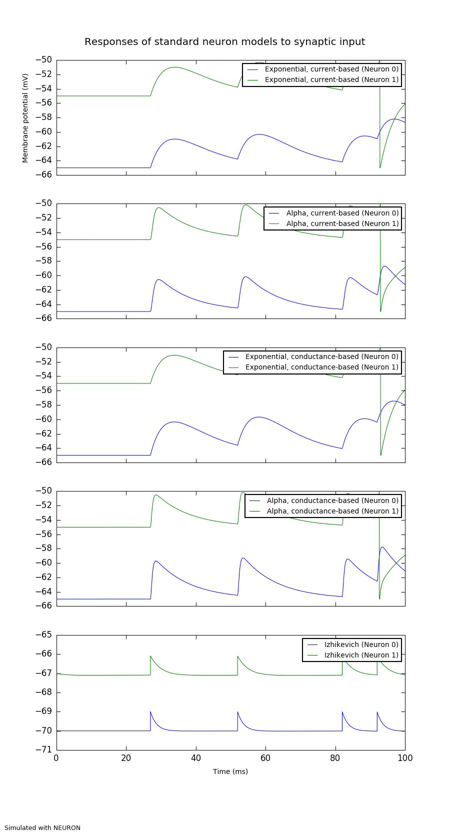
A demonstration of the responses of different standard neuron models to synaptic input.
This should show that for the current-based synapses, the size of the excitatory
post-synaptic potential (EPSP) is constant, whereas for the conductance-based
synapses it depends on the value of the membrane potential.
Usage: python synaptic_input.py [-h] [--plot-figure] [--debug] simulator
positional arguments:
simulator neuron, nest, brian or another backend simulator
optional arguments:
-h, --help show this help message and exit
--plot-figure Plot the simulation results to a file.
--debug Print debugging information
"""
from quantities import ms
from pyNN.utility import get_simulator, init_logging, normalized_filename
# === Configure the simulator ================================================
sim, options = get_simulator(("--plot-figure", "Plot the simulation results to a file.", {"action": "store_true"}),
("--debug", "Print debugging information"))
if options.debug:
init_logging(None, debug=True)
sim.setup(timestep=0.01, min_delay=1.0)
# === Build and instrument the network =======================================
# for each cell type we create two neurons, one of which we depolarize with
# injected current
cuba_exp = sim.Population(2, sim.IF_curr_exp(tau_m=10.0, i_offset=[0.0, 1.0]),
initial_values={"v": [-65, -55]}, label="Exponential, current-based")
cuba_alpha = sim.Population(2, sim.IF_curr_alpha(tau_m=10.0, i_offset=[0.0, 1.0]),
initial_values={"v": [-65, -55]}, label="Alpha, current-based")
coba_exp = sim.Population(2, sim.IF_cond_exp(tau_m=10.0, i_offset=[0.0, 1.0]),
initial_values={"v": [-65, -55]}, label="Exponential, conductance-based")
coba_alpha = sim.Population(2, sim.IF_cond_alpha(tau_m=10.0, i_offset=[0.0, 1.0]),
initial_values={"v": [-65, -55]}, label="Alpha, conductance-based")
v_step_izh = sim.Population(2, sim.Izhikevich(i_offset=[0.0, 0.002]),
initial_values={"v": [-70, -67], "u": [-14, -13.4]}, label="Izhikevich")
all_neurons = cuba_exp + cuba_alpha + coba_exp + coba_alpha + v_step_izh
try:
v_step_if = sim.Population(2, sim.IF_curr_delta(tau_m=10.0, i_offset=[0.0, 1.0]),
initial_values={"v": [-65, -55]}, label="Voltage step")
except NotImplementedError:
v_step_if = None
else:
all_neurons += v_step_if
# we next create a spike source, which will emit spikes at the specified times
spike_times = [25, 50, 80, 90]
stimulus = sim.Population(1, sim.SpikeSourceArray(spike_times=spike_times), label="Input spikes")
# now we connect the spike source to each of the neuron populations, with differing synaptic weights
connections = [sim.Projection(stimulus, population,
connector=sim.AllToAllConnector(),
synapse_type=sim.StaticSynapse(weight=w, delay=2.0),
receptor_type="excitatory")
for population, w in zip(all_neurons.populations, [1.6, 4.0, 0.03, 0.12, 2.0, 4.0])]
# finally, we set up recording of the membrane potential
all_neurons.record('v')
# === Run the simulation =====================================================
sim.run(100.0)
# === Calculate the height of the first EPSP =================================
print("Height of first EPSP:")
for population in all_neurons.populations:
# retrieve the recorded data
vm = population.get_data().segments[0].filter(name='v')[0]
# take the data between the first and second incoming spikes
vm12 = vm.time_slice(spike_times[0] * ms, spike_times[1] * ms)
# calculate and print the EPSP height
for channel in (0, 1):
v_init = vm12[:, channel][0]
height = vm12[:, channel].max() - v_init
print(" {:<30} at {}: {}".format(population.label, v_init, height))
# === Save the results, optionally plot a figure =============================
filename = normalized_filename("Results", "synaptic_input", "pkl", options.simulator)
all_neurons.write_data(filename, annotations={'script_name': __file__})
if options.plot_figure:
from pyNN.utility.plotting import Figure, Panel
figure_filename = filename.replace("pkl", "png")
panels = [
Panel(cuba_exp.get_data().segments[0].filter(name='v')[0],
ylabel="Membrane potential (mV)",
data_labels=[cuba_exp.label], yticks=True, ylim=(-66, -50)),
Panel(cuba_alpha.get_data().segments[0].filter(name='v')[0],
data_labels=[cuba_alpha.label], yticks=True, ylim=(-66, -50)),
Panel(coba_exp.get_data().segments[0].filter(name='v')[0],
data_labels=[coba_exp.label], yticks=True, ylim=(-66, -50)),
Panel(coba_alpha.get_data().segments[0].filter(name='v')[0],
data_labels=[coba_alpha.label], yticks=True, ylim=(-66, -50)),
Panel(v_step_izh.get_data().segments[0].filter(name='v')[0],
xticks=True, xlabel="Time (ms)",
data_labels=[v_step_izh.label], yticks=True, ylim=(-71, -65))
]
if v_step_if:
panels.insert(-1,
Panel(v_step_if.get_data().segments[0].filter(name='v')[0],
data_labels=[v_step_if.label], yticks=True, ylim=(-66, -50)),
)
Figure(
*panels,
title="Responses of standard neuron models to synaptic input",
annotations="Simulated with %s" % options.simulator.upper()
).save(figure_filename)
print(figure_filename)
# === Clean up and quit ========================================================
sim.end()