Data handling

Todo

add a note that data handling has changed considerably since 0.7, and give link to detailed changelog.

Recorded data in PyNN is always associated with the Population or Assembly from which it was recorded. Data may either be written to file, using the write_data() method, or retrieved as objects in memory, using get_data().

Retrieving recorded data

Handling of recorded data in PyNN makes use of the Neo package, which provides a common Python data model for neurophysiology data (whether real or simulated).

The get_data() method returns a Neo Block object. This is the top-level data container, which contains one or more Segments. Each Segment is a container for data sharing a common time basis - a new Segment is added every time the reset() function is called.

A Segment can contain lists of AnalogSignal and SpikeTrain objects. These data objects inherit from NumPy’s array class, and so can be treated in further processing (analysis, visualization, etc.) in exactly the same way as NumPy arrays, but in addition they carry metadata about units, sampling interval, etc.

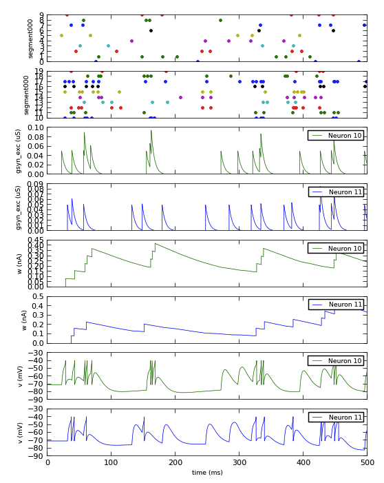
Here is a complete example of recording and plotting data from a simulation:

import pyNN.neuron as sim  # can of course replace `neuron` with `nest`, `brian`, etc.
import matplotlib.pyplot as plt
import numpy as np

sim.setup(timestep=0.01)
p_in = sim.Population(10, sim.SpikeSourcePoisson(rate=10.0), label="input")
p_out = sim.Population(10, sim.EIF_cond_exp_isfa_ista(), label="AdExp neurons")

syn = sim.StaticSynapse(weight=0.05)
random = sim.FixedProbabilityConnector(p_connect=0.5)
connections = sim.Projection(p_in, p_out, random, syn, receptor_type='excitatory')

p_in.record('spikes')
p_out.record('spikes')                    # record spikes from all neurons
p_out[0:2].record(['v', 'w', 'gsyn_exc'])  # record other variables from first two neurons

sim.run(500.0)

spikes_in = p_in.get_data()
data_out = p_out.get_data()

fig_settings = {
    'lines.linewidth': 0.5,
    'axes.linewidth': 0.5,
    'axes.labelsize': 'small',
    'legend.fontsize': 'small',
    'font.size': 8
}
plt.rcParams.update(fig_settings)
plt.figure(1, figsize=(6, 8))


def plot_spiketrains(segment):
    for spiketrain in segment.spiketrains:
        y = np.ones_like(spiketrain) * spiketrain.annotations['source_id']
        plt.plot(spiketrain, y, '.')
        plt.ylabel(segment.name)
        plt.setp(plt.gca().get_xticklabels(), visible=False)


def plot_signal(signal, index, colour='b'):
    label = "Neuron %d" % signal.annotations['source_ids'][index]
    plt.plot(signal.times, signal[:, index], colour, label=label)
    plt.ylabel("%s (%s)" % (signal.name, signal.units._dimensionality.string))
    plt.setp(plt.gca().get_xticklabels(), visible=False)
    plt.legend()


n_panels = sum(a.shape[1] for a in data_out.segments[0].analogsignals) + 2
plt.subplot(n_panels, 1, 1)
plot_spiketrains(spikes_in.segments[0])
plt.subplot(n_panels, 1, 2)
plot_spiketrains(data_out.segments[0])
panel = 3
for array in data_out.segments[0].analogsignals:
    for i in range(array.shape[1]):
        plt.subplot(n_panels, 1, panel)
        plot_signal(array, i, colour='bg'[panel % 2])
        panel += 1
plt.xlabel("time (%s)" % array.times.units._dimensionality.string)
plt.setp(plt.gca().get_xticklabels(), visible=True)

plt.show()

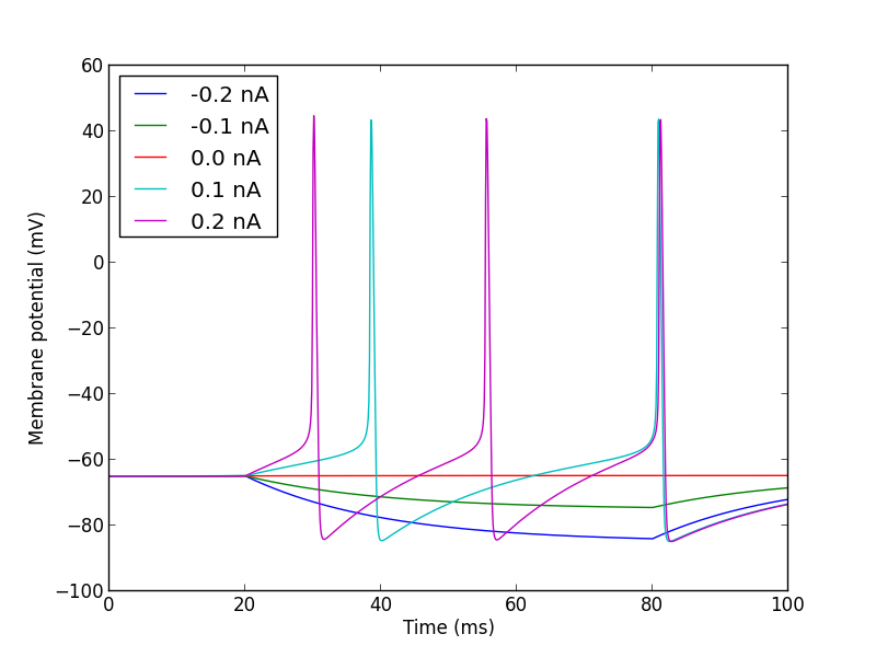
The adoption of Neo as an output representation also makes it easier to handle data when running multiple simulations with the same network, calling reset() between each run. In previous versions of PyNN it was necessary to retrieve the data before every reset(), and take care of storing the resulting data. Now, each run just creates a new Neo Segment, and PyNN takes care of storing the data until it is needed. This is illustrated in the example below.

import pyNN.neuron as sim  # can of course replace `nest` with `neuron`, `brian`, etc.
import matplotlib.pyplot as plt
from quantities import nA

sim.setup()

cell = sim.Population(1, sim.HH_cond_exp())
step_current = sim.DCSource(start=20.0, stop=80.0)
step_current.inject_into(cell)

cell.record('v')

for amp in (-0.2, -0.1, 0.0, 0.1, 0.2):
    step_current.amplitude = amp
    sim.run(100.0)
    sim.reset(annotations={"amplitude": amp * nA})

data = cell.get_data()

sim.end()

for segment in data.segments:
    vm = segment.analogsignals[0]
    plt.plot(vm.times, vm,
             label=str(segment.annotations["amplitude"]))
plt.legend(loc="upper left")
plt.xlabel("Time (%s)" % vm.times.units._dimensionality)
plt.ylabel("Membrane potential (%s)" % vm.units._dimensionality)

plt.show()

Note

if you still want to retrieve the data after every run you can do so: just call get_data(clear=True)

Writing data to file

Neo provides support for writing to a variety of different file formats, notably an assortment of text-based formats, NumPy binary format, Matlab .mat files, and HDF5. To write to a given format, we create a Neo IO object and pass it to the write_data() method:

>>> from neo.io import NixIO
>>> io = NixIO(filename="my_data.h5")
>>> population.write_data(io)

As a shortcut, for file formats with a well-defined file extension, it is possible to pass just the filename, and PyNN will create the appropriate IO object for you:

>>> population.write_data("my_data.mat")  # writes to a Matlab file

By default, all the variables that were specified in the record() call will be saved to file, but it is also possible to save only a subset of the recorded data:

>>> population.write_data(io, variables=('v', 'gsyn_exc'))

When running distributed simulations using MPI (see Running parallel simulations), by default the data is gathered from all MPI nodes to the master node, and only saved to file on the master node. If you would prefer that each node saves its own local subset of the data to disk separately, use gather=False:

>>> population.write_data(io, gather=False)

Saving data to a file does not delete the data from the Population object. If you wish to do so (for example to release memory), use clear=True:

>>> population.write_data(io, clear=True)

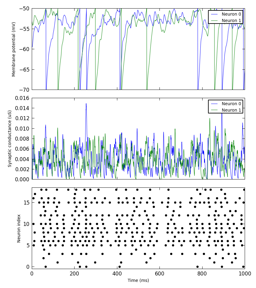
Simple plotting

Plotting Neo data with Matplotlib, as shown above, can be rather verbose, with a lot of repetitive boilerplate code. PyNN therefore provides a couple of classes, Figure and Panel, to make quick-and-easy plots of recorded data. It is possible to customize the plots to some extent, but for publication-quality or highly-customized plots you should probably use Matplotlib or some other plotting package directly.

A simple example:

from pyNN.utility.plotting import Figure, Panel

...

population.record('spikes')
population[0:2].record(('v', 'gsyn_exc'))

...

data = population.get_data().segments[0]

vm = data.filter(name="v")[0]
gsyn = data.filter(name="gsyn_exc")[0]

Figure(
    Panel(vm, ylabel="Membrane potential (mV)"),
    Panel(gsyn, ylabel="Synaptic conductance (uS)"),
    Panel(data.spiketrains, xlabel="Time (ms)", xticks=True)
).save("simulation_results.png")

Other packages for working with Neo data

A variety of software tools are available for working with Neo-format data, for example SpykeViewer and OpenElectrophy.