NEST

Configuration options

Continuous time spiking

In traditional simulation schemes spikes are constrained to an equidistant time grid. However, for some neuron models, NEST has the capability to represent spikes in continuous time.

At setup the user can choose the continuous time scheme

setup(spike_precision='off_grid')

or the conventional grid-constrained scheme

setup(spike_precision='on_grid')

where ‘off_grid’ is the default.

The following PyNN standard models have an off-grid implementation: IF_curr_exp, SpikeSourcePoisson EIF_cond_alpha_isfa_ista.

Todo

add a list of native NEST models with off-grid capability

Here is an example showing how to specify the option in a PyNN script and an illustration of the different outcomes:

import numpy as np
from pyNN.nest import *
import matplotlib.pyplot as plt


def test_sim(on_or_off_grid, sim_time):
    setup(timestep=1.0, min_delay=1.0, max_delay=1.0, spike_precision=on_or_off_grid)
    src = Population(1, SpikeSourceArray(spike_times=[0.5]))
    cm = 250.0
    tau_m = 10.0
    tau_syn_E = 1.0
    weight = cm / tau_m * np.power(tau_syn_E / tau_m, -tau_m / (tau_m - tau_syn_E)) * 20.5
    nrn = Population(1, IF_curr_exp(cm=cm, tau_m=tau_m, tau_syn_E=tau_syn_E,
                                    tau_refrac=2.0, v_thresh=20.0, v_rest=0.0,
                                    v_reset=0.0, i_offset=0.0))
    nrn.initialize(v=0.0)
    prj = Projection(src, nrn, OneToOneConnector(), StaticSynapse(weight=weight))
    nrn.record('v')
    run(sim_time)
    return nrn.get_data().segments[0].analogsignals[0]


sim_time = 10.0
off = test_sim('off_grid', sim_time)
on = test_sim('on_grid', sim_time)


def plot_data(pos, on, off, ylim, with_legend=False):
    ax = plt.subplot(1, 2, pos)
    ax.plot(off.times, off, color='0.7', linewidth=7, label='off-grid')
    ax.plot(on.times, on, 'k', label='on-grid')
    ax.set_ylim(*ylim)
    ax.set_xlim(0, 9)
    ax.set_xlabel('time [ms]')
    ax.set_ylabel('V [mV]')
    if with_legend:
        plt.legend()


plot_data(1, on, off, (-0.5, 21), with_legend=True)
plot_data(2, on, off, (-0.05, 2.1))
plt.show()

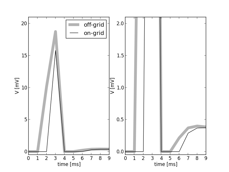
The gray curve shows the membrane potential excursion in response to an input spike arriving at the neuron at t = 1.5 ms (left panel, the right panel shows an enlargement at low voltages). The amplitude of the post-current has an unrealistically high value such that the threshold voltage for spike generation is crossed. The membrane potential is recorded in intervals of 1 ms. Therefore the first non-zero value is measured at t = 2 ms. The threshold is crossed somewhere in the interval (3 ms, 4 ms], resulting in a voltage of 0 at t = 4 ms. The membrane potential is clamped to 0 for 2 ms, the refractory period. Therefore, the neuron recovers from refractoriness somewhere in the interval (5 ms, 6 ms] and the next non-zero voltage is observed at t = 6 ms. The black curve shows the results of the same model now integrated with a grid constrained simulation scheme with a computation step size of 1 ms. The input spike is mapped to the next grid position and therefore arrives at t = 2 ms. The first non-zero voltage is observed at t = 3 ms. The output spike is emitted at t = 4 ms and this is the time at which the membrane potential is reset. Consequently, the model neuron returns from refractoriness at exactly t = 6 ms. The next non-zero membrane potential value is observed at t = 7 ms.

The following publication describes how the continuous time mode is implemented in NEST and compares the performance of different approaches:

Hanuschkin A, Kunkel S, Helias M, Morrison A and Diesmann M (2010) A general and efficient method for incorporating precise spike times in globally time-driven simulations. Front. Neuroinform. 4:113. doi:10.3389/fninf.2010.00113

Random number generator

To set the seed for the NEST random number generator:

setup(rng_seed=12345)

You can also choose the type of RNG:

setup(rng_type="Philox_32", rng_seed=12345)

Using native cell models

To use a NEST neuron model with PyNN, we wrap the NEST model with a PyNN NativeCellType class, e.g.:

>>> from pyNN.nest import native_cell_type, Population, run, setup
>>> setup()
0
>>> ht_neuron = native_cell_type('ht_neuron')
>>> poisson = native_cell_type('poisson_generator')
>>> p1 = Population(10, ht_neuron(Tau_m=20.0))
>>> p2 = Population(1, poisson(rate=200.0))

We can now initialize state variables, set/get parameter values, and record from these neurons as from standard cells:

>>> p1.get('Tau_m')
20.0
>>> p1.get('Tau_theta')
2.0
>>> p1.get('C_m')
Traceback (most recent call last):
...
NonExistentParameterError: C_m (valid parameters for ht_neuron are:
  AMPA_E_rev, AMPA_Tau_1, AMPA_Tau_2, AMPA_g_peak, E_K, E_Na, GABA_A_E_rev,
  GABA_A_Tau_1, GABA_A_Tau_2, GABA_A_g_peak, GABA_B_E_rev, GABA_B_Tau_1,
  GABA_B_Tau_2, GABA_B_g_peak, KNa_E_rev, KNa_g_peak, NMDA_E_rev, NMDA_Sact,
  NMDA_Tau_1, NMDA_Tau_2, NMDA_Vact, NMDA_g_peak, NaP_E_rev, NaP_g_peak,
  T_E_rev, T_g_peak, Tau_m, Tau_spike, Tau_theta, Theta_eq, g_KL, g_NaL,
  h_E_rev, h_g_peak, spike_duration)
>>> p1.initialize(V_m=-70.0, Theta=-50.0)
>>> p1.record('V_m')
>>> run(250.0)
250.0
>>> output = p1.get_data()

To connect populations of native cells, you need to know the available synaptic receptor types:

>>> ht_neuron.receptor_types
['NMDA', 'AMPA', 'GABA_A', 'GABA_B']
>>> from pyNN.nest import Projection, AllToAllConnector
>>> connector = AllToAllConnector()
>>> prj_ampa = Projection(p2, p1, connector, receptor_type='AMPA')
>>> prj_nmda = Projection(p2, p1, connector, receptor_type='NMDA')

Using native synaptic plasticity models

To use a NEST STDP model with PyNN, we use the native_synapse_type() function:

>>> from pyNN.nest import native_synapse_type
>>> stdp = native_synapse_type("stdp_synapse")(**{"Wmax": 50.0, "lambda": 0.015})
>>> prj_plastic = Projection(p1, p1, connector, receptor_type='AMPA', synapse_type=stdp)

Common synapse properties

Some NEST synapse models (e.g. stdp_facetshw_synapse_hom) make use of common synapse properties to conserve memory. This has the following implications for their usage in PyNN:

• Common properties can only have one homogeneous value per projection. Trying to assign heterogeneous values will result in a ValueError.

• Common properties can currently not be retrieved using Projection.get. However, they will only deviate from the default when changed manually.