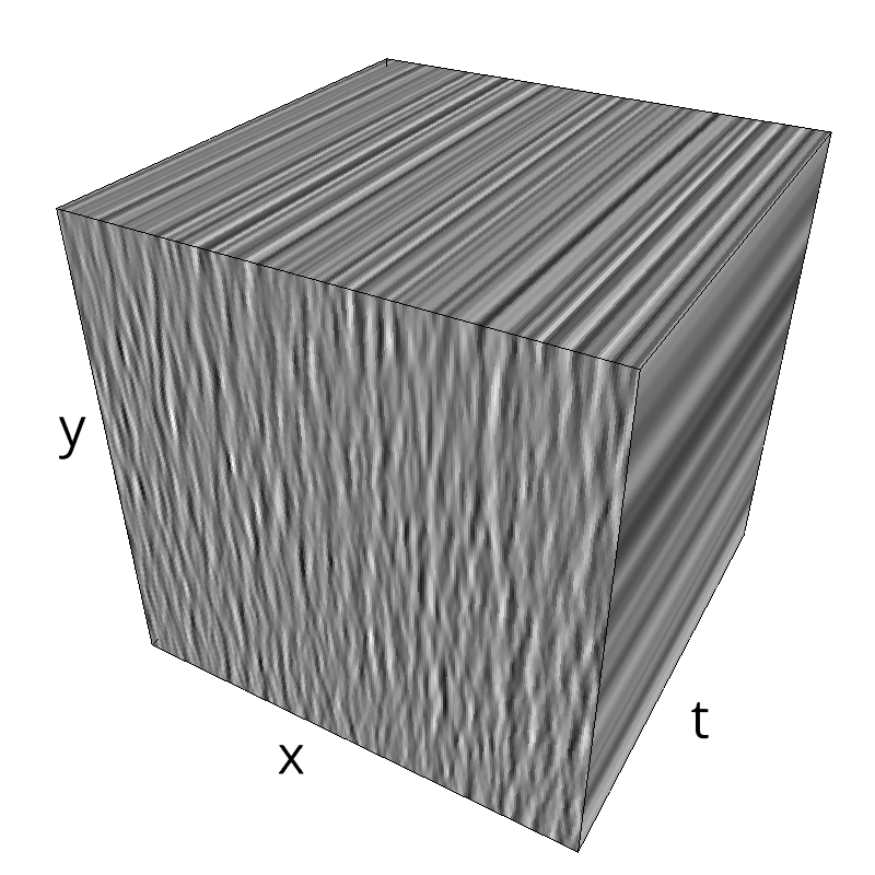
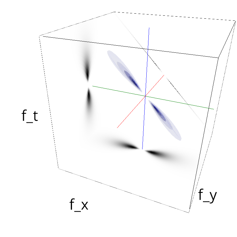
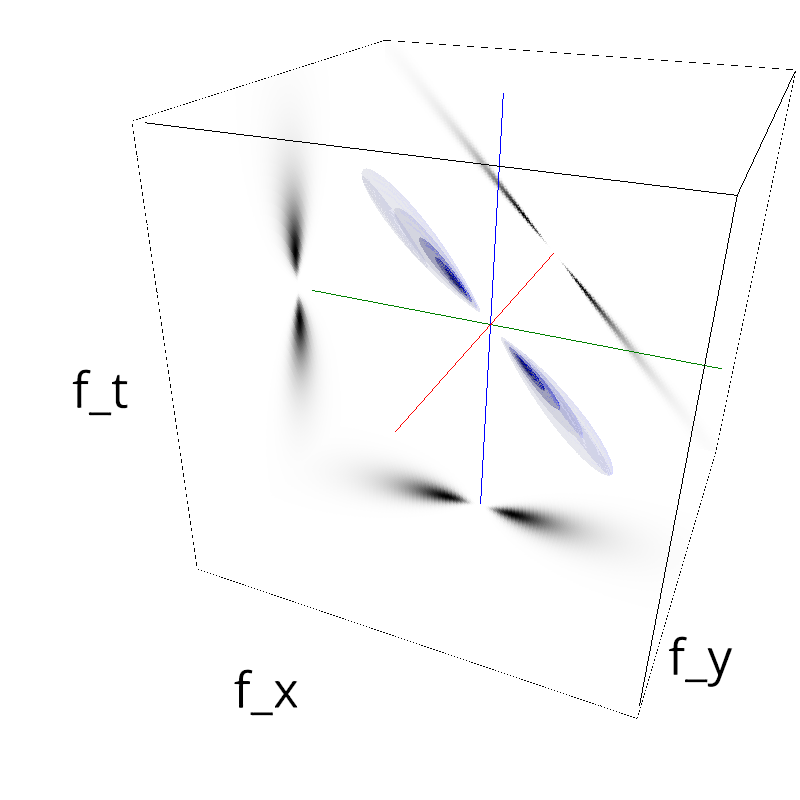
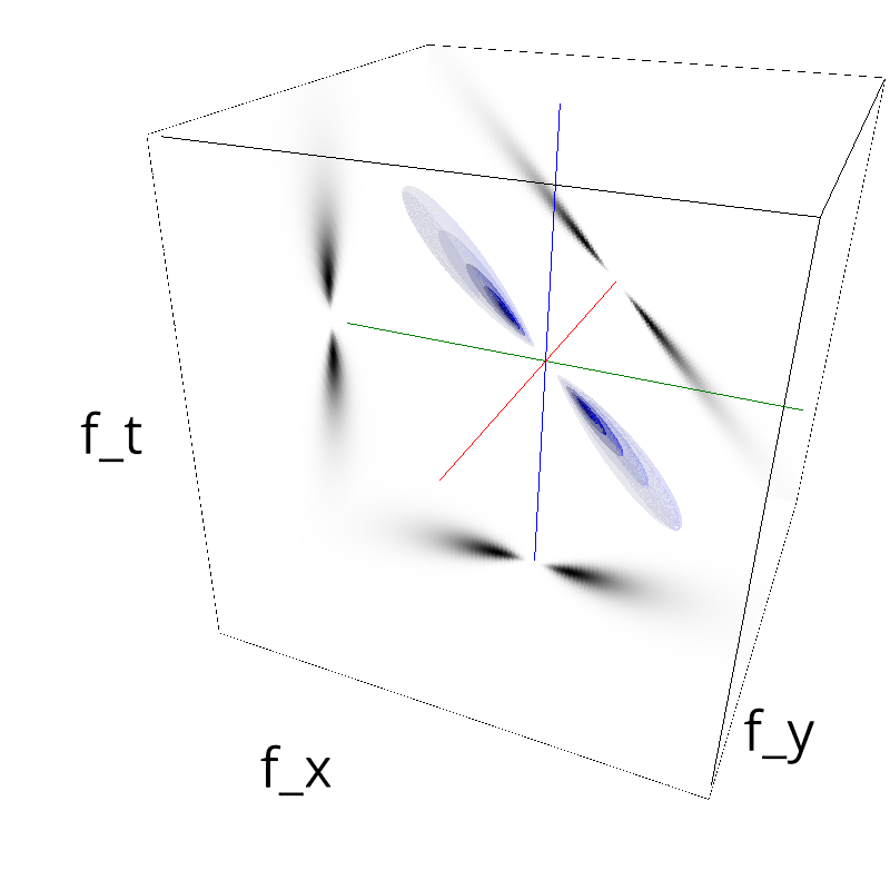
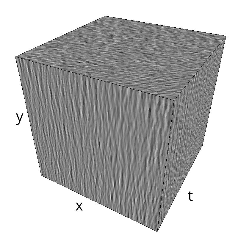
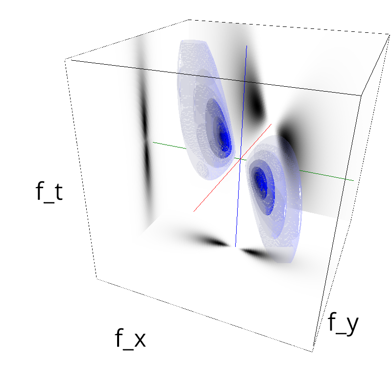
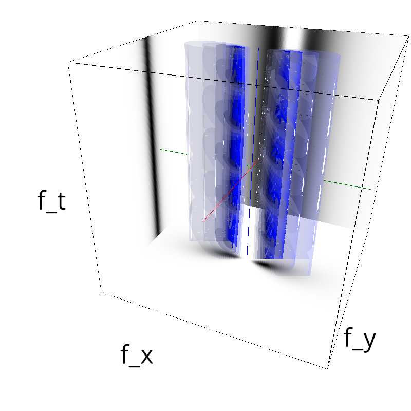
Testing Speed
Testing the Speed
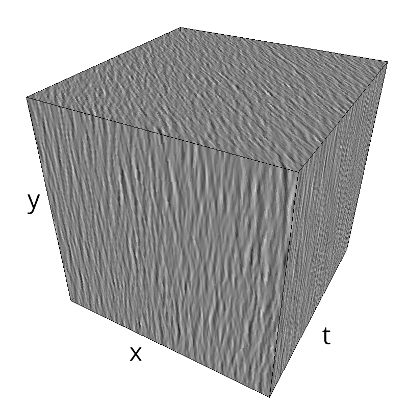
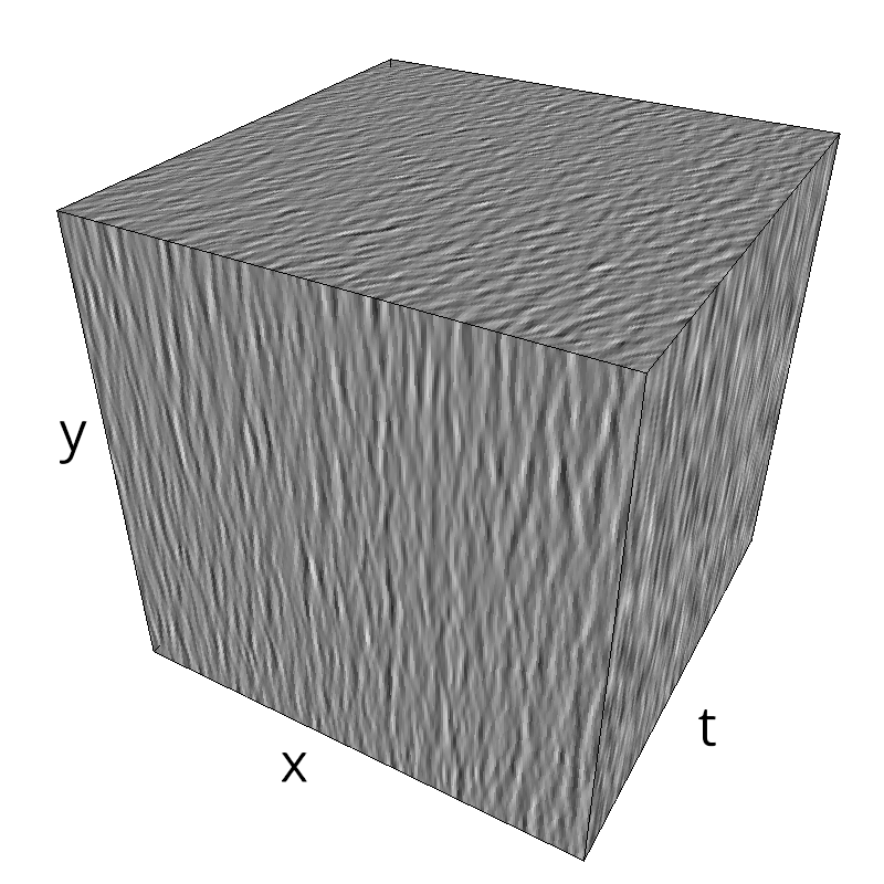
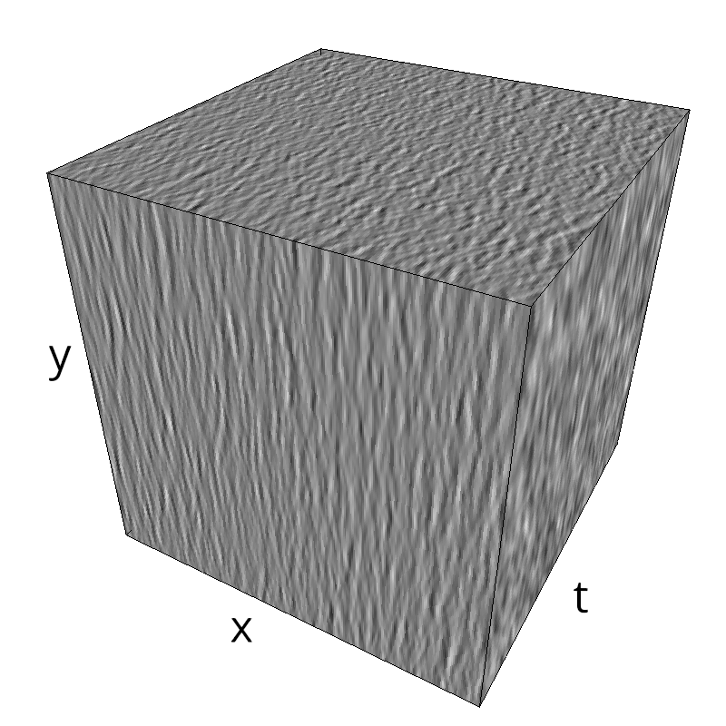
A moving pattern (stimulus/image) can be thought as a set of pixels and that each pixel intensities are translated from one frame to the next frame (the intensities, not the pixel:
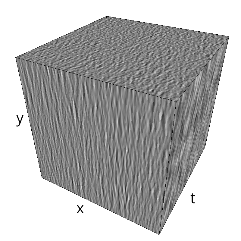
I(x,t)=I(x+u,t+1); space is a vector with coordinates (x1,x2)’ and time is t. u=(u1,u2) is the 2D velocity. Motion Clouds represent 2D + t images. x(t), each pixel follows a 2D path as a function of time. So we have a space-time function f(x,t) by translating a 2D signal f0(x) with velocity u, i.e, f(x,t)=f0(x-ut).
The Fourier transform of such a function is
F(wx, wy, wt)=F0(wx,wy) \delta(u1wx + u2wy + wt)
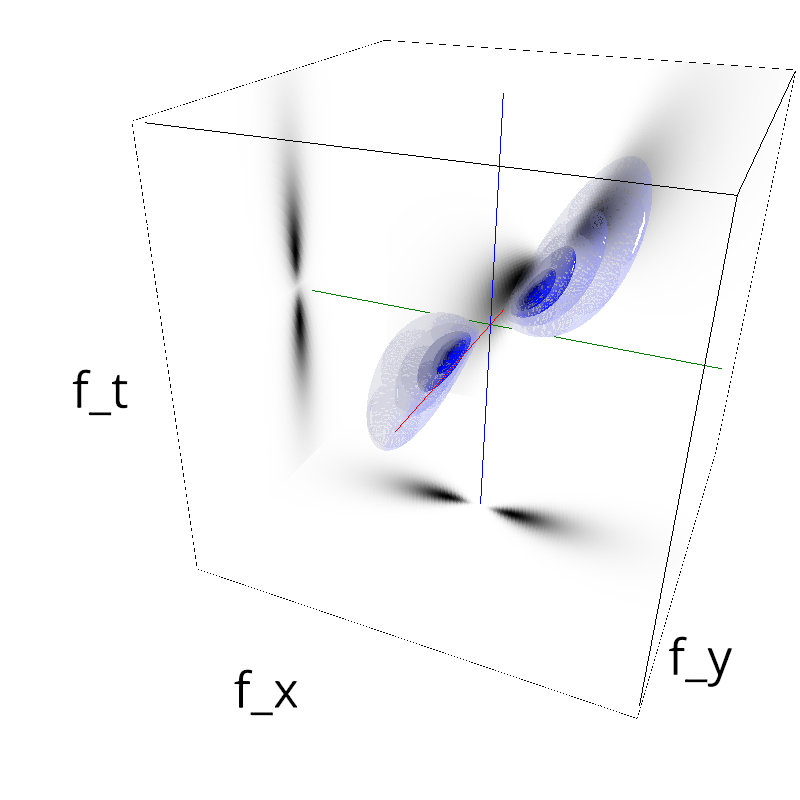
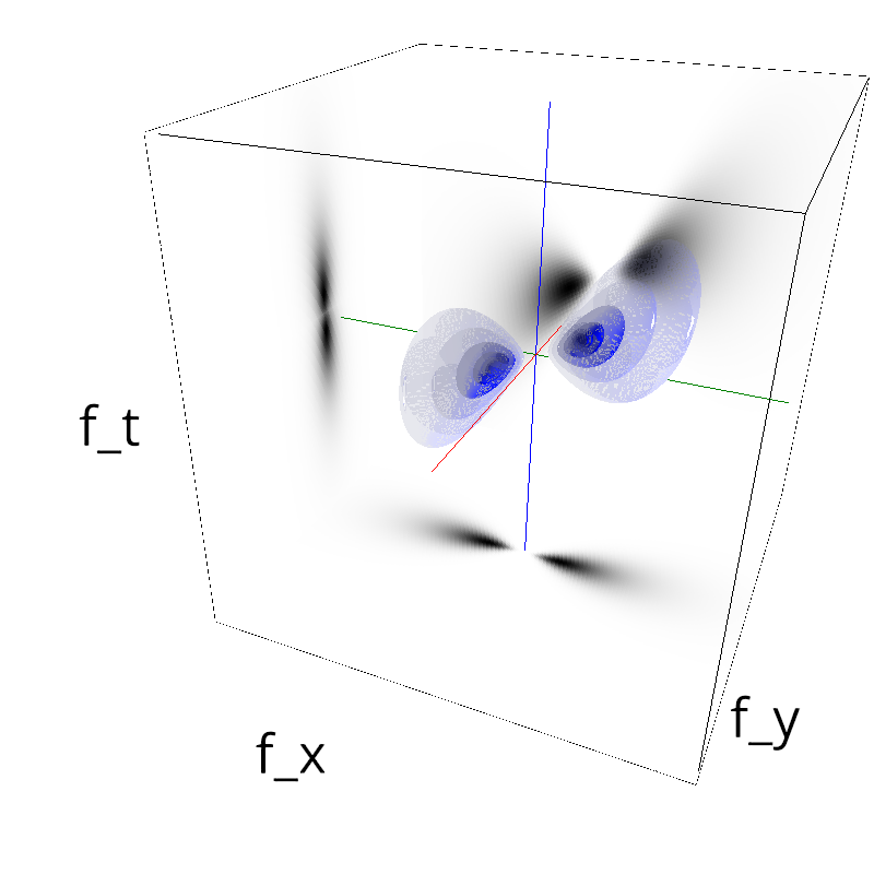
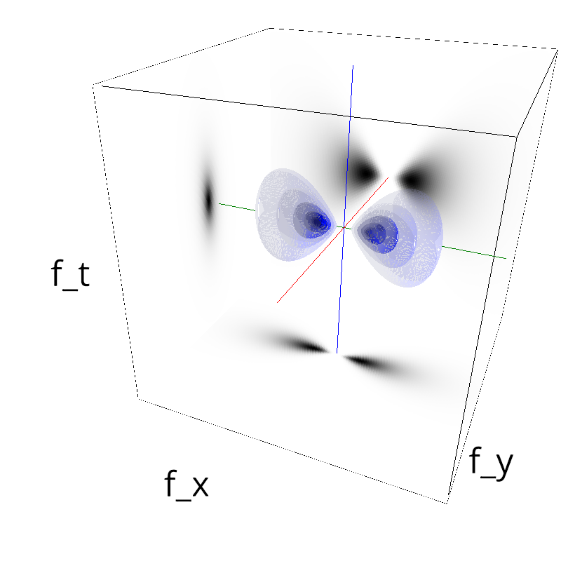
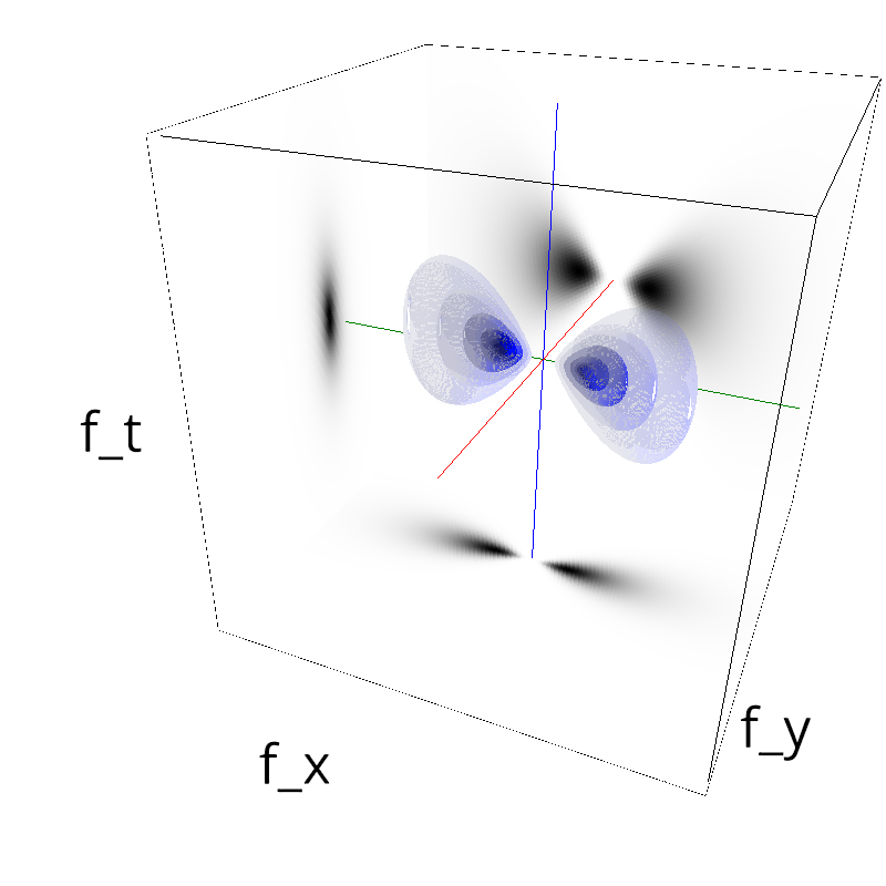
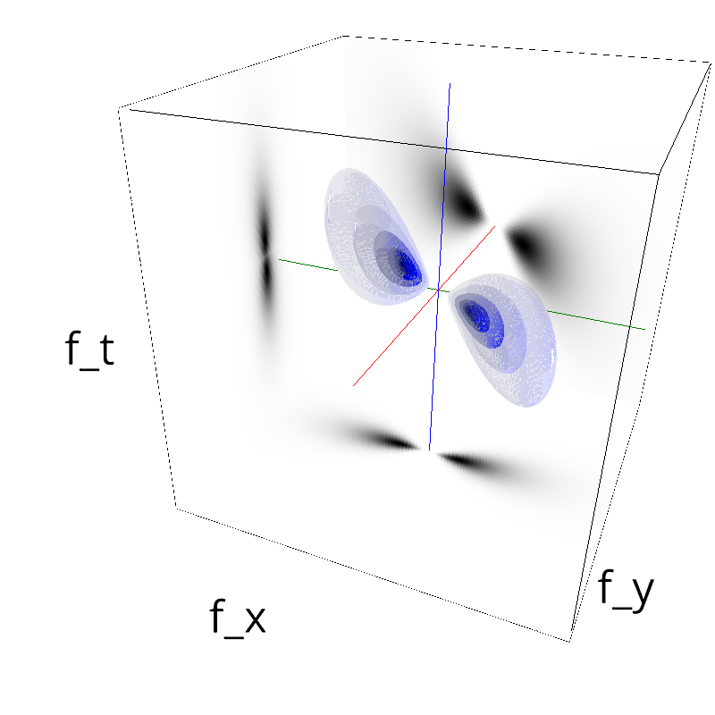
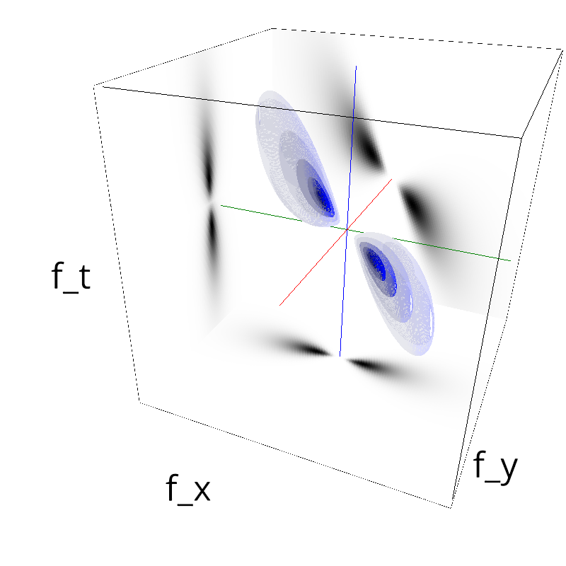
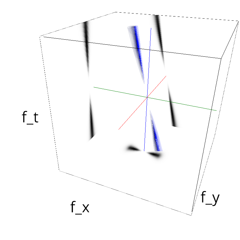
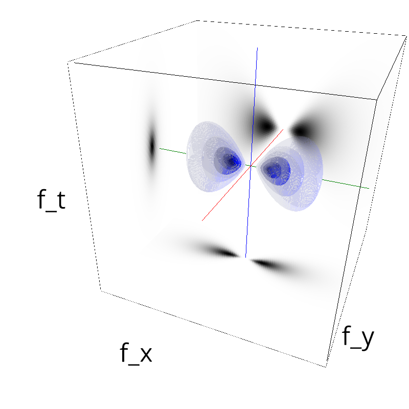
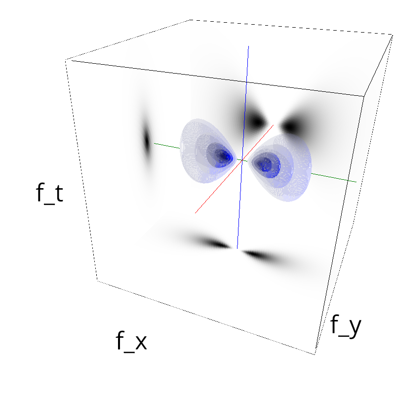
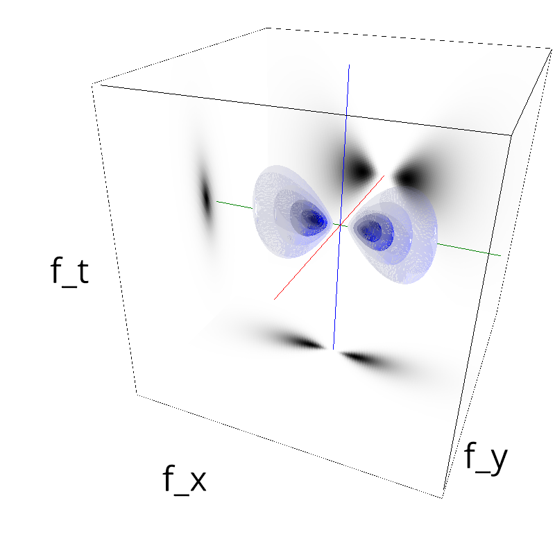
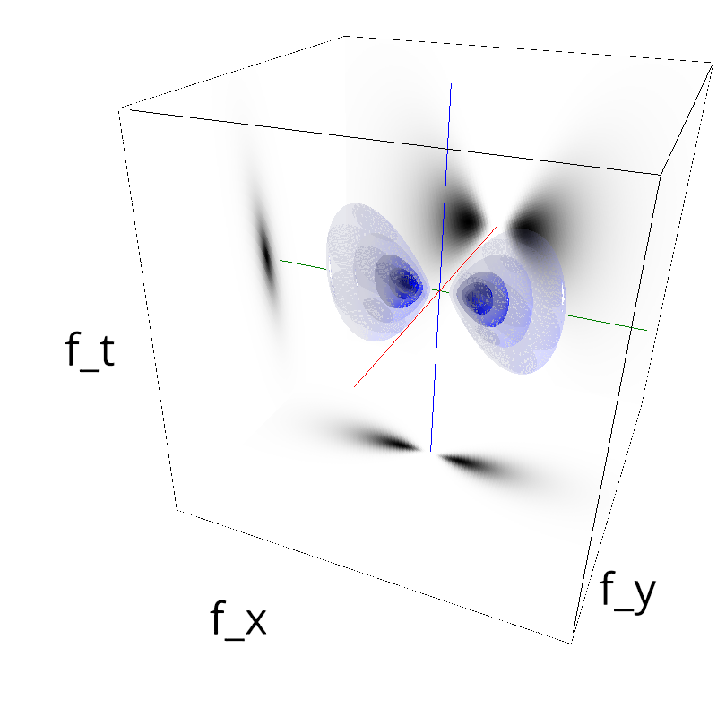
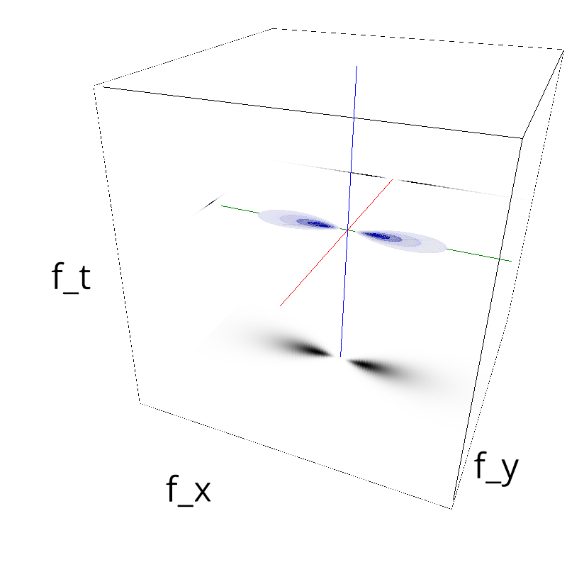
F0 is the 2D transform of f0 and \delta is the dirac delta. The energy spectrum is nonzero on a plane whose orientation gives the velocity.
In [1]:
%matplotlib inline
import numpy as np
np.set_printoptions(precision=3, suppress=True)
import pylab
import matplotlib.pyplot as plt
#!rm -fr ../files/speed*
In [2]:
import MotionClouds as mc
name = 'speed'
fx, fy, ft = mc.get_grids(mc.N_X, mc.N_Y, mc.N_frame)
help(mc.envelope_speed)
In [3]:
# explore parameters
for V_X in [-1.0, -0.5, 0.0, 0.1, 0.5, 1.0, 4.0]:
    name_ = name + '-V_X-' + str(V_X).replace('.', '_')
    z = mc.envelope_gabor(fx, fy, ft, V_X=V_X)
    mc.figures(z, name_)
    mc.in_show_video(name_)
In [4]:
for V_Y in [-1.0, -0.5, 0.5, 1.0, 2.0]:
    name_ = name + '-V_Y-' + str(V_Y).replace('.', '_')
    z = mc.envelope_gabor(fx, fy, ft, V_X=0.0, V_Y=V_Y)
    mc.figures(z, name_)
    mc.in_show_video(name_)
In [5]:
for B_V in [0, 0.001, 0.01, 0.05, 0.1, 0.5, 1.0, 10.0]:
    name_ = name + '-B_V-' + str(B_V).replace('.', '_')
    z = mc.envelope_gabor(fx, fy, ft, B_V=B_V)
    mc.figures(z, name_)
    mc.in_show_video(name_)
