Continuous time spike interaction

In traditional simulation schemes spikes are constrained to an equidistant time grid. However, some simulators have the capability to represent spikes in continuous time or to switch between the two modes.

At setup the user can choose the continuous time scheme:

setup(spike_precision='off_grid')

or the conventional grid-constrained scheme:

setup(spike_precision='on_grid')

where ‘on_grid’ is the default.

PyNN requires the grid-constrained implementation of a neuron model. If ‘off_grid’ is chosen but a continuous time implementation of a specific neuron model is not available, the grid-constrained version is used. If ‘off_grid’ is chosen but the backend does not support the continuous time scheme at all, an error is generated.

The following continuous time implementations are available:

IF_curr_alpha	in prep.
IF_curr_exp	x
IF_cond_alpha
IF_cond_exp
HH_cond_exp
EIF_cond_alpha_isfa_ista	in prep.

Here is an example showing how to specify the option in a PyNN script and an illustration of the different outcomes:

from pyNN.nest import *
from matplotlib.pyplot import *
def test_sim(on_or_off_grid, sim_time):
    setup(timestep=1.0, min_delay=1.0, max_delay=1.0, spike_precision=on_or_off_grid)
    src = Population(1, SpikeSourceArray, cellparams={'spike_times': [0.5]})
    cm        = 250.0
    tau_m     =  10.0
    tau_syn_E =   1.0
    weight    = cm/tau_m * numpy.power(tau_syn_E/tau_m, -tau_m/(tau_m-tau_syn_E)) * 20.5
    nrn = Population(1, IF_curr_exp, cellparams={'cm':         cm,
                                                 'tau_m':      tau_m,
                                                 'tau_syn_E':  tau_syn_E,
                                                 'tau_refrac':  2.0,
                                                 'v_thresh':   20.0,
                                                 'v_rest':      0.0,
                                                 'v_reset':     0.0,
                                                 'i_offset':    0.0})
    nrn.initialize('v', 0.0)
    prj = Projection(src, nrn, OneToOneConnector(weights=weight))
    nrn.record_v()
    run(sim_time)
    Vm = nrn.get_v()
    end()
    return numpy.transpose(Vm)[1:3]
sim_time = 10.0
off = test_sim('off_grid', sim_time)
on  = test_sim('on_grid', sim_time)
subplot(1,2,1)
plot(off[0], off[1],color='0.7',linewidth=7, label='off-grid')
plot(on[0], on[1],'k', label='on-grid')
ylim(-0.5,21)
xlim(0,9)
xlabel('time [ms]')
ylabel('V [mV]')
legend()
subplot(1,2,2)
plot(off[0],off[1],color='0.7',linewidth=7)
plot(on[0],on[1],'k')
ylim(-0.05,2.1)
xlim(0,9)
xlabel('time [ms]')
ylabel('V [mV]')
show()

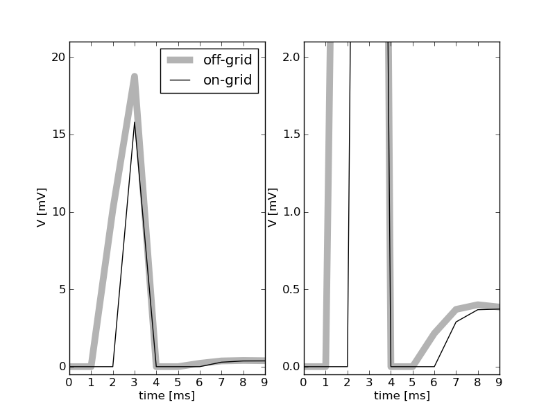
The gray curve shows the membrane potential excursion in response to an input spike arriving at the neuron at t=1.5ms (left panel, the right panel shows an enlargement at low voltages). The amplitude of the post-current has an unrealistically high value such that the threshold voltage for spike generation is crossed. The membrane potential is recorded in intervals of 1ms. Therefore the first non-zero value is measured at t=2ms. The threshold is crossed somewhere in the interval (3ms,4ms], resulting in a voltage of 0 at t=4ms. The membrane potential is clamped to 0 for 2ms, the refractory period. Therefore, the neuron recovers from refractoriness somewhere in the interval (5ms,6ms] and the next non-zero voltage is observed at t=6ms. The black curve shows the results of the same model now integrated with a grid constrained simulation scheme with a computation step size of 1ms. The input spike is mapped to the next grid position and therefore arrives at t=2ms. The first non-zero voltage is observed at t=3ms. The output spike is emitted at t=4ms and this is the time at which the membrane potential is reset. Consequently, the model neuron returns from refractoriness at exactly t=6ms. The next non-zero membrane potential value is observed at t=7ms.

The following publication describes how the continuous time mode is implemented in NEST and compares the performance of different approaches:

Hanuschkin A, Kunkel S, Helias M, Morrison A and Diesmann M (2010) A general and efficient method for incorporating precise spike times in globally time-driven simulations. Front. Neuroinform. 4:113. doi: 10.3389/fninf.2010.00113.